A Typical courses on Calculus will contain a rudimentary introduction to series. But one might ask why study them at all? Instead of providing an answer to this question, I will be showing why they are interesting in the first place, which might motivate further investigations in some future post.
A mathematical series is the countable infinite sum of arbitrary objects(numbers, functions, etc.). In this post we will be focusing on series of real numbers. Consider the series $$1 + 2 + 3 + \cdots$$ Leaving aside Ramanujan’s summation, this series clearly diverges to infinity. Notationally, we write
$$\sum_{n=1}^{\infty}{a_n} = a_1 + a_2 + a_3 + \cdots$$
where $a_n = n$ for all $n \in \mathbb{N}$. It goes without saying that the choice of $a_n$ in not restricted to any particular number. A better behaved series is the series given by
$$\sum_{n=1}^{\infty}{\frac{1}{2^{n-1}}} = 1 + \frac{1}{2} + \frac{1}{4} + \frac{1}{8}+\cdots$$ which is an example of a geometric series. Such series are known to converge when the absolute value of the common factor is less than $1$, which is $\frac{1}{2}$ in this case. But what does it mean for a series to converge?
Before discussing the convergence of series, we need to define sequences and their convergence. In simple terms, a sequence is an an ordered list of infinite size. We have already seen two sequences in this post: $(1,2,3, \cdots)$ and $(1, \frac{1}{2},\frac{1}{4}, \frac{1}{8}, \cdots)$. We now define convergence: the sequence $(s_n)$ converges to a limit $L$ if for every arbitrarily small $\epsilon >0$, we can look far enough into the sequence and find a term $s_N$ for which any term $s_n$ succeeding this $N^{th}$ term, the inequality $|s_n-L|<\epsilon$ holds. In other words, as we progress through the sequence, the distance between terms and the limit $L$ diminishes.
With a firm definition of sequences in hand, we define the convergence of series. The series $\sum_{n=1}^{\infty}{a_n}$ is said to be convergent if the sequence of partial sums $(s_n)$, defined by $$s_m = a_1 + a_2 + \dots + a_m,$$ for all $m \in \mathbb{N}$ is convergent.
Going back to our geometric series example, we can write out the sequence of partial sums as $$(1,\ 1.5,\ 1.75,\ 1.875,\ 1.9375, 1.96875, \cdots).$$ Figure 1 shows numeric estimates of the partial sums $s_m$ for $m = 1,2,3, \dots,1000$. Before stating any conclusions about the convergence of this geometric series, it is important to note that numerical convergence does not imply convergence due to limitations on computer precision. However, it is well established that this geometric series converges to $2$.
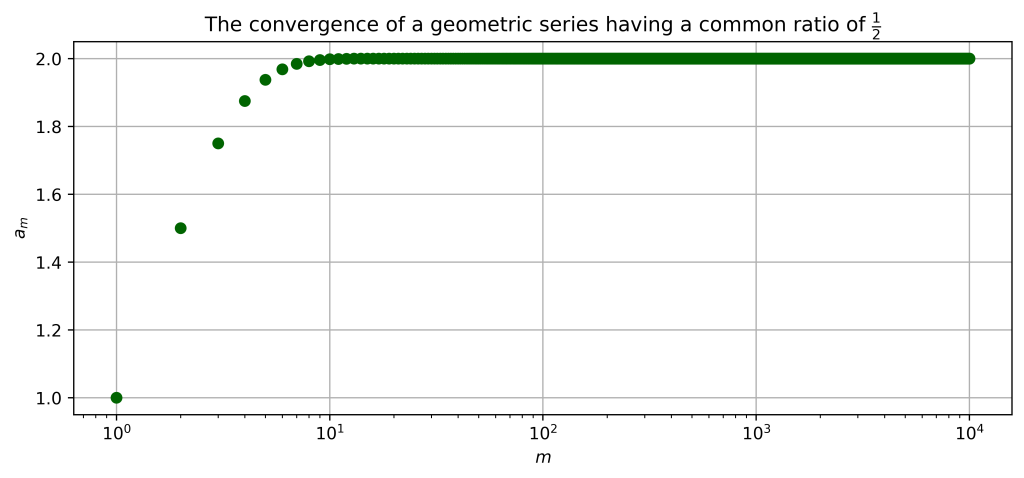
$$\text{Figure 1: Numerical solution to} \sum_{n=0}^{\infty} \left({\frac{1}{2}} \right)^n$$ To gain a more intuitive understanding on how this series converges to $2$, consider using the slider found in the illustration in figure 2. The grey box has an area of $2$ units, and by adding the infinite terms(blue boxes) of the series, the total area occupied by the blue boxes will approach that of the grey box.
$$\text{Figure 2: Geometric solution to} \sum_{n=0}^{\infty} \left({\frac{1}{2}} \right)^n$$
Similarly, we can write out a geometric series having a $1/3$ common factor.
$$\sum_{n=0}^{\infty} \left({\frac{1}{3}} \right)^n = 1 + \frac{1}{3} + \frac{1}{9} + \frac{1}{27} + \cdots$$ Figure 3 shows numeric estimates of the partial sums $s_m$ for $m = 1,2,3, \dots,1000$, which shows that the series converges to $3/2$. Similar to before, figure 4 gives a geometric interpretation to this convergence. However, its interpretation slightly differs: we start with a rectangle having an area equal to $3$ units, and then fill the terms of the series, twice. This way, two copies of the geometric series will cover a total area of $3$ units, which suggests that one series will cover an area of $3/2$ units.
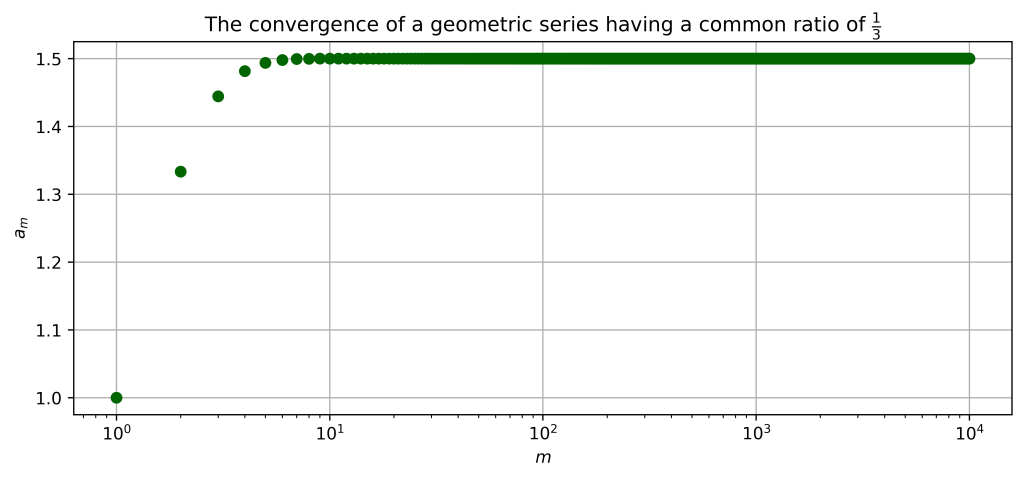
$$\text{Figure 3: Numerical solution to} \sum_{n=0}^{\infty} \left({\frac{1}{3}} \right)^n$$
$$\text{Figure 4: Geometric solution to} \sum_{n=0}^{\infty} \left({\frac{1}{3}} \right)^n$$ The geometric series having a common ratio of $1/4$, written as
$$\sum_{n=0}^{\infty} \left({\frac{1}{4}} \right)^n = 1 + \frac{1}{4} + \frac{1}{16} + \frac{1}{64} + \cdots,$$ converges to $4/3$ as per figure 5. Moreover, it has its own unique geometric interpretation involving triangles instead of rectangles. In figure 6, we start with an Isosceles triangle having an area of $4$ units and then overlay the terms(colored triangles) of the geometric series on top, three times for each term. By simple geometry, each successive triangle will have an area one fourth that of it’s predecessor. This way, three copies of the geometric series will fill up the grey triangle. This suggests that one copy of the geometric series will have a total area of $4/3$ units.
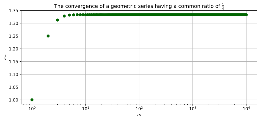
$$\text{Figure 5: Numerical solution to} \sum_{n=0}^{\infty} \left({\frac{1}{4}} \right)^n$$
$$\text{Figure 6: Geometric solution to} \sum_{n=0}^{\infty} \left({\frac{1}{4}} \right)^n$$
In all these geometrical interpretations, we made use of the self-similarity of the shapes; a topic heavily studied in fractal geometry. It turns out that geometric series are called geometric for this exact reason.
In application, geometric series are computed using a known equation, which will be derived below. Consider the fact that $1-x^{n+1}$ could be written as a telescoping series given by
$$(1-x^{n+1}) = (1-x)(1+x+x^2+\cdots+x^n)$$
We rearrange terms to obtain
$$1+x+x^2+\cdots+x^n = \frac{1-x^{n+1}}{1-x}$$ Equivalently,
$$\sum_{k=0}^{n}{x}^k = \frac{1-x^{n+1}}{1-x}$$
Therefore,
$$
\begin{aligned}
\sum_{k=0}^{\infty}{x}^k &= \lim_{n\rightarrow \infty}{\sum_{k=0}^{n}{x}^k} \\
&= \lim_{n\rightarrow \infty}{\frac{1-x^{n+1}}{1-x}} \\
&= {\frac{1-\lim_{n\rightarrow \infty}(x^{n+1})}{1-x}}
\end{aligned}
$$
When $|x| <1$, it follows that $\lim_{n\rightarrow \infty}(x^{n+1}) = 0$. This makes
$$\sum_{k=0}^{\infty}{x}^k = \frac{1-0}{1-x} = \frac{1}{1-x}.$$
The ease of computing the value of geometric series lead to their adoption in a wide variety of fields. It is used in solving for recursions in computer algorithms and is helpful in proving some mathematics theorems.
Leave a Reply